Overview
Asymptotic Notation is used to describe the represent time complexity of an algorithm where it represents time taken to execute the algorithm for a given input, n.
The following are some of the major notation systems:
- Big O is used for the worst case running time.
- Big Theta (Θ) is used when the running time is the same for all cases.
- Big Omega (Ω) is used for the best case running time.
Out of the three, Big O notation is widely used. Besides Big O notation can also be used to represent space complexity where it represents memory consumption.
Details
Big O, pronounced as Big Oh, is commonly referred to as Order of. It is a way to express the upper bound of an algorithm’s time complexity, since it analyses the worst-case situation of algorithm. It provides an upper limit on the time taken by an algorithm in terms of the size of the input represented as n.
For a given input of n, time complexity of various algorithms can be categorized under Big O notation as below. The performance ratio is represented as input : time.
| Name | Notation | Description | Example |
|---|---|---|---|
| Constant | O(1) | Time taken is constant. | Assignments System function calls |
| Logarithmic | O(log n) | Time increases linearly in 1:0.5 ratio. | Binary search |
| Linear | O(n) | Time increases linearly in 1:1. | Find an entry from an unsorted array |
| Log Linear | O(n log (n)) | Time increases linearly in 1:1.5. | Quick sort |
| Polynomial | O(n^c) | Time increases as a polynomial in 1:n^c ratio where c can be 2 for quadric, 3 for cubic etc. | Selection Sort [ O(n^2) ]. |
| Exponential | O(c^n) | Time increases exponentially in 1:c^n ratio where c can be 2 or higher. | Print all subsets of a given Set or Array [ O(2^n) ]. |
| Factorial | O(n!) | Time increases factorially with n | Permutations of a set. |
The following chart graphically compares big o variations.

The following table compares input size vs time for various time complexities.

There are many ways to compute an algorithms time complexity.
In case of simple algorithms, by counting each code statement that's executed. It can be simple assignment statements, if-else branches, switch statements, loops, system function calls etc.
It can be assumed that each statement is associated with a certain number of execution unit or eu.
For example, assignments, or system function calls can be considered that it takes 1 eu.
In case of if-else , it's 2 eus based on the check.
The eu of a block of code can be considered as an aggregate of eu of individual statements. However some variations apply on case to case basis.
Time complexity of an algorithm is calculated based on number of eus it generates for an input n.
Time is represents actual time taken to execute the algorithm. It can be represented as a polynomial expression such as a*n^b + c*n^d +...+z.
The highest degree of the polynomial expression is considered for big O notation.
It's discussed in detail below.
| Code | Execution Units | Category |
|---|---|---|
i=10; v[20]=20;int_vector.at(10)=5; | 1 1 1 2 1 1 1 | Constant O(1) |
for (int i=64; i>=1; i/=2) { intlist.push_back(i); intlist2.push_back(i); }for (int i=1; i<64; i*=2) { intlist.push_back(i); intlist2.push_back(i); } | 3*log2(64)+4 8 7 7 3*log2(64)+1 7 6 6 | Logarithmic O(log n) |
| 3*sqrt(64)+1 9 8 8 | square root O(sqrt(n)) |
| 3n+1 (n+1) n n | Linear O(n) |
| 2n^2+2n+1 n+1 n*(n+1) n*n | Polynomial O(n^2) |
| 2^5-1 31 15 15 | Exponential O(2^n) |
string s("abc"); permute(s);void permute(string& s, int idx=0) { static int len = s.size()-1; if (idx == len) { return; } for (int i = idx; i < s.size(); i++) { swap(s[idx], s[i]); permute(s, idx + 1); swap(s[idx], s[i]); } } | 6*3!+17 10 6 10 9 9 9 | Factorial O(n!) |
In case of recursive algorithms, the above method can be overwhelming. In such cases number of calls generated or number of comparisons or number of swaps can be substituted to compute time complexity.
constant O(1)
An algorithm is considered as constant time when it takes a constant time to execute irrespective of input.
Consider the table below.
The assignment statements are considered to take O(1).
The function call at() take O(1) as it can be assumed that time taken to assign a value to an element in a 10 item array or vector is same as 1000 item array or vector.
In all these cases, input size has no effect and therefore constant time complexity can be represented as O(1).

logarithmic O(log n)
The time taken to execute an logarithmic algorithms for an input n is comparable to log2(n) in the worst case.
Binary search algorithm takes O(log n) as shown in the tree diagram below. The data set contains integers [20,30,40,50,80,90,100]. To search value is 40 takes takes 3 comparisons, [0,6], [0,2] and [2,2]

Consider the following code that performs binary search. There are two for loops. The first loop creates a vector of sizes 7,14, and 21 and populates them with serial numbers. The second loop performs the binary search of a number not in range thus triggering worst case scenario.
vector<string> comps;
int bs(int *data, int val, int low, int high)
{
    if ( low < 0 || low > high)
        return -1;
    int m = (low+high)/2;
    comps.push_back(string("[") + to_string(low) + "," + to_string(high) + "]");
    if (val == data[m])
        return m;
    else if (val < data[m])
        return bs(data, val, low, m-1);
    else if (val > data[m])
        return bs(data, val, m+1, high);
}

for (int i = 1; i < 4; ++i)
{
    vector<int> v(7*i);
    iota(begin(v),end(v),1);
    for (auto i:v) cout << i << " ";
    cout << endl;
    comps.clear();
    bs(v.data(), 50, 0, v.size()-1);
    sort(begin(comps),end(comps),[](const string& a, const string& b){return (a.length() < b.length());});
    for (auto i:comps) cout << i << " ";
    cout << endl << endl;
}
The time complexity of the single call to bs() can be considered as an amortized constant. The t number of compares in each case can be approximated as time.
When n = 7, 3 compares are performed thus time = 3 or O(3) or approximately O(log 7).
When n = 14, 4 compares are performed thus time = 4 or O(4) or approximately O(log 14).
When n = 21, 5 compares are performed thus time = 5 or O(5) or approximately O(log 21).
In general Logarithmic time can be represented as O(log n).

linear O(n)
The time taken to execute an linear algorithms for an input n is comparable to n in the worst case.
Consider the following code that performs find operation on unsorted array.
There are two for loops. The first loop creates a vector of sizes 7,14, and 21 and populates them with randomly ordered numbers. The second loop performs find operation of a random number on them.
vector<string> swaps;
int knt=0;
int find(int *data, int val, int low, int high)
{
    for (int i=low; i<=high; ++i)
    {
        knt++;
        swaps.push_back(string("[") + to_string(data[i]) + "," + to_string(val) +  "]");
        if (data[i] == val)
        {
            return i;
        }
    }
    return -1;
}


for (int i = 1; i < 4; ++i)
{
    knt = 0;
    vector<int> v(7*i);
    iota(begin(v),end(v),1);
    shuffle(begin(v), end(v), default_random_engine(2018));
    for (auto i:v) cout << i << " ";
    cout << endl;
    swaps.clear();
    int n = v.size()-1;
    find(v.data(), v[n-rand()%3], 0, n);
    sort(begin(swaps),end(swaps),[](const string& a, const string& b){return (a.length() < b.length());});
    for (auto i:swaps) cout << i << " ";
    cout << endl;
    cout << "# compares:" << knt;
    cout << endl << endl;

}
The time complexity of the single call to find() can be considered as an amortized constant. The t number of compares in each case can be approximated as time.
When n = 7, 6 compares are performed thus time = 6 or O(6) or approximately O(7).
When n = 14, 13 compares are performed thus time = 13 or O(13) or approximately O(14).
When n = 21, 21 compares are performed thus time = 21 or O(21) or approximately O(21).
In general linear time can be represented as O(n).

log linear O(n log n)
The time taken to execute an log linear algorithms for an input n is comparable to n * log2(n) in the worst case.
Quick sort algorithm takes O(nlog n) as shown in the tree diagram below. The data set contains integers [9,-3,5,2,6,8,-6,1,3]. To sort , 16 comparisons were performed as shown below.
[9,3] [5,3] [2,3] [6,3] [8,3] [1,3] [2,1] [8,6] [5,6] [9,6] [9,8] [-3,3] [-6,3] [-3,1] [-6,1] [-3,-6]

Consider the following code that performs quick sort.
There are two for loops. The first loop creates a vector of sizes 5,10, and 15 and populates them with randomly ordered numbers. The second loop performs partition sort on them.
vector<string> comps;
int knt = 0, knt2=0;
void swap(int &l, int &r)
{
    ++knt2;
    swap<int>(l, r);
}

int  partition( int *data, int low, int high)
{
    int ltpvt = low - 1;
    for (int i=low; i<high; ++i)
    {
        ++knt;
        comps.push_back(string("[") + to_string(data[i]) + "," + to_string(data[high])  + "]");
        if (data[i] < data[high])
        {

            ++ltpvt;
            if (i != ltpvt)
                swap(data[i], data[ltpvt]);
        }
    }
    ++ltpvt;
    if (high != ltpvt)
        swap(data[high], data[ltpvt]);
    return ltpvt;
}

void qs(int *data, int low, int high, int n)
{
    if (low >= high)
        return;

    int pi = partition(data,low,high);
    qs(data,low, pi-1,n);
    qs(data,pi+1,high,n);
}

    for (int i=1; i<4; ++i)
    {
        vector<int>  v(5*i);
        iota(begin(v),end(v),1);
        shuffle(begin(v), end(v), default_random_engine(2018));

        knt = 0;
        knt2 = 0;
        for (auto i:v) cout << i << " "; cout << endl;
        comps.clear();
        qs(v.data(),0,v.size()-1,v.size());
        sort(begin(comps),end(comps),[](const string& a, const string& b){return (a.length() < b.length());});
        for (auto i:comps) cout << i << " "; cout << endl;
        for (auto i:v) cout << i << " "; cout << endl;
        cout << "# swaps:" << knt2 << endl;
        cout << "# compares:" << knt << endl;
        cout << endl;
    }
The time complexity of the single call to qs() can be considered as an amortized constant. The t number of compares in each case can be approximated as time.
When n = 5, 10 compares are performed thus time = 10 or O(10) or approximately O(5log 5).
When n = 10, 32 compares are performed thus time = 32 or O(32) or approximately O(10log10).
When n = 15, 41 compares are performed thus time = 41 or O(41) or approximately O(15log15).
In general log linear time can be represented as O(nlog n).

polynominal O(n^2)
The time taken to execute a polynomial algorithms for an input n is comparable to n^ 2 in the worst case.
Consider the following code that performs selection sort.
There are two for loops. The first loop creates a vector of sizes 5,10, and 15 and populates them with randomly ordered numbers. The second loop performs partition sort on them.
vector<string> comps;
int knt = 0, knt2=0;
void swap(int &l, int &r)
{
    ++knt2;
    swap<int>(l, r);
}

void ss(int *data, int low, int high, int n)
{
    for (int i=low; i < high; ++i)
    {
        int k=i;
        for (int j=i+1; j <= high; ++j)
        {
            ++knt;
            comps.push_back(string("[")+to_string(data[k])+","+to_string(data[j])+"]");
            if (data[k] > data[j])
            {
                k = j;
            }

        }
        if (k != i)
            swap(data[i], data[k]);
    }
}
    for (int i=1; i<4; ++i)
    {
        vector<int>  v(5*i);
        iota(rbegin(v),rend(v),1);
        shuffle(begin(v), end(v), default_random_engine(2018));

        knt = 0;
        knt2 = 0;
        for (auto i:v) cout << i << " "; cout << endl;
        comps.clear();
        ss(v.data(),0,v.size()-1,v.size());
        sort(begin(comps),end(comps),[](const string& a, const string& b){return (a.length() < b.length());});
        for (auto i:comps) cout << i << " "; cout << endl;
        for (auto i:v) cout << i << " "; cout << endl;
        cout << "# compares:" << knt << endl;
        cout << "# swaps:" << knt2 << endl;
        cout << endl;
    }
The time complexity of the single call to ss() can be considered as an amortized constant. The t number of compares in each case can be approximated as time.
When n = 5, 10 compares are performed thus time = 10 or O(10) or approximately O(5^2).
When n = 10, 45 compares are performed thus time = 45 or O(45) or approximately O(10^2).
When n = 15, 105 compares are performed thus time = 105 or O(105) or approximately O(15^2).
In general polynomial time can be represented as O(n^2).

Exponential O(k^n)
The time taken to execute a exponential algorithms for an input n is comparable to k^ n in the worst case where k can be 2, 3 etc.
For example, Backtracking algorithm to find subsets takes O(k^n).
In the example below, the data set contains integers [1,2,3]. The algorithm produces 8 subsets as shown below. [] [3] [2] [1] [23] [13] [12] [123]. Its time complexity can be calculated as 2^3.

Consider the following code that prints all possible subsets of a set.
There are two for loops. The first loop creates a vector of sizes 4,5,6 and populates them with randomly ordered characters. The second loop finds the subsets and prints them.
vector<string> subsets;
int knt = 0;
void FindSubsets(const string& arr, int index, string& currentSubset)
{

    if (index >= arr.size())
    {
        knt++;
        subsets.push_back("[" + currentSubset + "] ");
        return;
    }

    string temp(currentSubset);
    FindSubsets(arr, index + 1, temp);

    currentSubset.push_back(arr[index]);
    FindSubsets(arr, index + 1, currentSubset);
}


    for (int i=1; i<4; ++i)
    {
        string currentSubset;
        string  v(3+i,' ');
        iota(begin(v),end(v),'a');
        shuffle(begin(v), end(v), default_random_engine(2018));

        knt = 0;
        for (auto i:v) cout << i << " "; cout << endl;
        subsets.clear();
        FindSubsets(v,0,currentSubset);
        sort(begin(subsets), end(subsets),[](string& a, string& b){return a.size() < b.size();});
        for (auto i:subsets) cout << i;
        cout << endl;
        cout << "# subsets:" << knt << endl;
        cout << endl;
    }
The time complexity of the single call to FindSubsets() can be considered as an amortized constant. The t number of subsets generated in each case can be approximated as time.
When n = 4, 16 subsets are generated thus time = 16 or O(16) or approximately O(2^4).
When n = 5, 32 subsets are generated thus time = 32 or O(32) or approximately O(2^5).
When n = 6, 64 subsets are generated thus time = 64 or O(64) or approximately O(2^6).
In general Exponential time can be represented as O(k^n) where k=2.

Factorial O(n!)
The time taken to execute a exponential algorithms for an input n is comparable to n! in the worst case.
For example, Backtracking algorithm to find permutations takes O(n!).
In the example below, the data set contains letters [A,B,C]. The algorithm produces 6 permutations as shown below. [ABC] [ACB] [BAC] [BCA] [CBA] [CAB]. Its time complexity can be calculated as 3!.
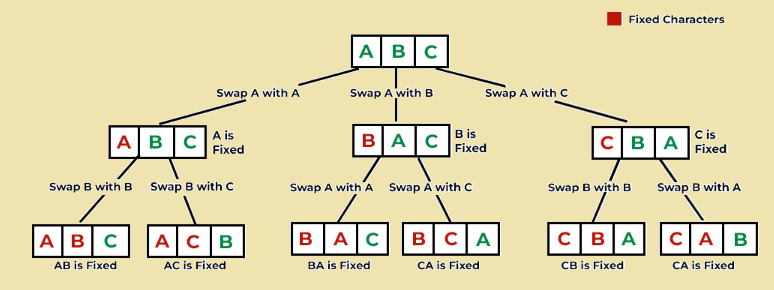
Consider the following code that prints all possible permutations of a set.
There are two for loops. The first loop creates a vector of sizes 3,4,5 and populates them with randomly ordered characters. The second loop finds permutations and prints them.
vector<string> permutations;
int knt = 0;
void FindPermutatons(const string& arr, int index)
{
    if (index >= arr.size())
    {
        knt++;
        permutations.push_back("[" + arr + "] ");
        return;
    }

    for (int i=index; i < arr.size(); ++i)
    {
        string temp(arr);
        swap(temp[i],temp[index]);
        FindPermutatons(temp, index + 1);
    }
}

    for (int i=1; i<4; ++i)
    {
        string  v(2+i,' ');
        iota(begin(v),end(v),'a');

        knt = 0;
        for (auto i:v) cout << i << " "; cout << endl;
        permutations.clear();
        FindPermutatons(v,0);
        sort(begin(permutations), end(permutations),[](string& a, string& b){return a.size() < b.size();});
        for (auto i:permutations) cout << i;
        cout << endl;
        cout << "# Permutatons:" << knt << endl;
        cout << endl;
    }
The time complexity of the single call to FindPermutatons() can be considered as an amortized constant. The t number of permutations generated in each case can be approximated as time.
When n = 3, 6 subsets are generated thus time = 6 or O(6) or approximately O(3!).
When n = 4 24 subsets are generated thus time = 24 or O(24) or approximately O(4!).
When n = 5, 120 subsets are generated thus time = 120 or O(120) or approximately O(5!).
In general factorial time can be represented as O(n!).

No comments:
Post a Comment